Porting (and emscripten’ing) some legacy code (>20 years old)
Posted by Neil in Uncategorized on March 19th, 2023
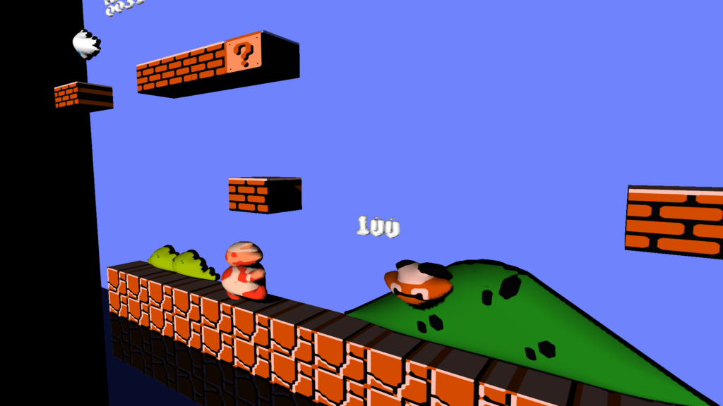
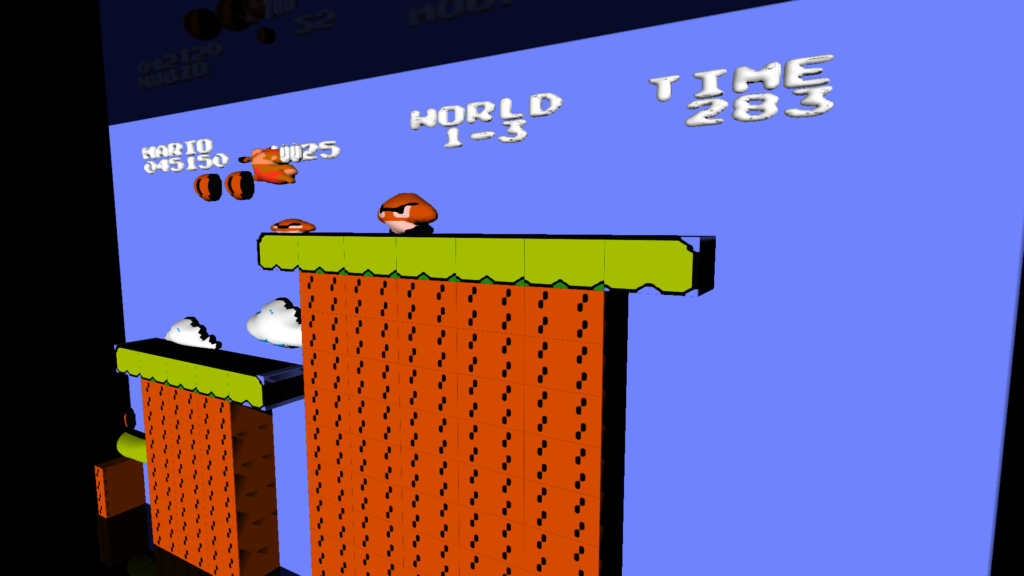
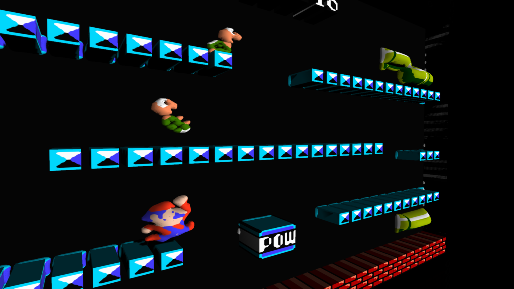
I have an old post (http://www.neilbirkbeck.com/?p=1066) that discussed some of the first Game clones that I had made when I was first starting to code (sometime in the early 2000s). At the time, I was using windows and must have been using some online tutorials for how to do DirectX Graphics.
A few weeks ago, I was interested in checking out some of that code to see how much effort it would be to port it over to Linux. In the back of my mind, I was also thinking it would be cool to get things running in the brower (using Emscripten). So when deciding which libraries to use for Linux, I wanted to make sure that I chose ones that would be compatible with Emscripten — if possible. Turns out SDL was supported.
Overall, the limited subset of DirectX that I was using very close to the APIs offered in SDL. So porting the first game (bomberman) was fairly easy and maybe only took a few hours of work for the first game. And since my “engine” was fairly similar, finishing the other games (which were made earlier) was fairly easy.
The code for the various projects is horrendous (it is over 20 years old now), and basically I had no idea what I was doing.
Projects
Bomberman
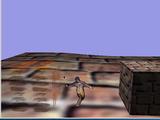
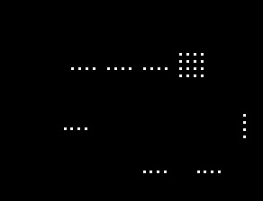
The first of the games that I ported over was Bomberman. There were some features that I didn’t bother with (e.g., there is also a music player that was using FMod Sound).
Bomberman even had some very primitive AI.
Bomberman even had a crude version of multiplayer. I remember at the time, I was heavily influenced by Quake 3. So I had a console where you could connect to a server. Unfortunately, there was no real synchronization between the game state — only the action was sent from client to server (and vice versa) so it was possible for the client and server to get out of sync. An example of what it looks like in the following video:
Once I had the Linux code working, it was surprisingly easy to get things working with Emscripten. The only hiccup was around setting up some library flags and debugging some the sleep function. It was the only thing that needed special handling. The Emscripted version looks like:
You can try it out here:
http://www.neilbirkbeck.com/legacy/emscripten/bman.html
Use ‘a’, ‘s’, ‘d’, and ‘w’ to move. And z/x to place bombs / explode them if you have the detonator.
Breakout
Next up was Breakout. Use the mouse to move the pad and press ‘ ‘ to release the ball. The default level has tonnes of powerups. This one was never completed (e.g., no title screens, etc.). This may have been the very first game…
Again, there is a terminal (press tilde) and there are a few commands (map, to set the level e.g., \map map1.txt, or \give ball.
http://www.neilbirkbeck.com/legacy/emscripten/arkanoid.html
Pacman
For pacman, I remember one of the “innovations” I had added is that you can use the space key to chew through the walls. The wall rendering is done for each frame so it was easily to update.
http://www.neilbirkbeck.com/legacy/emscripten/pacman.html
Titris
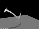
Last, but not least is titris — a tetris clone. Despite having written various versions of tetris. This was the first one. And was probably the first crack at any AI that I had. At the time, I remember thinking that AI was just a bunch of If/else statements. I basically had no idea what I was doing, but still came up with something that kind of worked. Press ‘p’ to test out the AI:
http://www.neilbirkbeck.com/legacy/emscripten/titris.html
Code
All the code is here. Be ware, I didn’t know what I was doing, and in porting the code to Linux all I did was clang-format (no real fixes).
A simple traffic simulator
Several years ago, while shopping in Target, I was thinking about making a simple traffic simulator. I’m not entirely sure what sparked the idea — I think at the time, I was interested in the effect that a few bad (or slow) drivers could have on traffic. Or maybe it was about how long it took for a traffic slow-down to clear up.
Anyway, when I was thinking of things to work on over this past Christmas break, this was one of the ideas that resurfaced. So I decided to poke around with it. Given that I forgot why I wanted to do it in the first place, I should have known it was going to be hard to decide on a reasonable end state for the project–and no I didn’t look to see what was out there.
I guess I got the simulator to the point where cars sped up, slowed down for other cars, slowed down for intersections (and corners), and randomly plotted their path (using updating estimates of speed for each of the road segments). I didn’t spend all that much time on the visualization, so it doesn’t look that great. Here’s a rendering, with some annotations below:
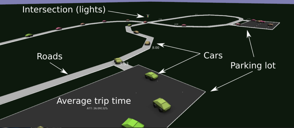
Overall, I guess there were some fun little problems to solve: like how to deal with intersections, implementing the smooth interpolation around corners, determining when to slow down, trying to make things more efficient, etc..
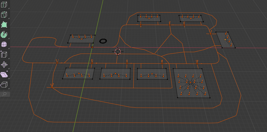
As usual, the level editor is in Blender, and it was kind of fun just setting up new levels (adding new roads, intersections, etc.) and watching the simulation to see what happened (when cars cut each other off, how it slows down traffic, and when cars start taking long routes due to traffic on shorter ones). Felt a bit like adult Lego.

I spent a bit of time optimizing the simulation, so I think it could simulate about 50K cars (in a single thread)…although I only ever added 1k cars.
Anyway, most of the features of the simulation plus some actual renderings from the simulator are in the following video (use the chapter annotations see interesting points)
Source code and some more details about the project here:https://github.com/nbirkbeck/dsim
Reinforcement-learned bike pumper
You don’t know me, but lately I’ve been getting super interested in learning to jump on a dirt jump bike. Like doing an ollie on a skateboard, there is lots of technique that experienced people have that makes them effective, confident, and able to jump high. I suspect that the details around this are not something that are easily communicated, and lots of it is becomes second nature (and is likely done by muscle-memory / feel).
I’ve been trying to see what gets you to go higher (e.g., https://youtu.be/wR2SI9WnNrw?t=17), but haven’t fully unlocked it yet.
Given that I’ve been playing around with reinforcement learning lately, I was curious if I could setup a simple environment and get an RL agent to learn how to pump in order to get maximum efficiency. I ended up not focusing on height, but rather pump-ability. I setup a small simulation to see if this was possible. I’m bad at physics, so one of the most challenging parts was to work some model of the “pump” into the physics model that was controllable by the agent…kind of like how we use our arms and legs to pump. I ended up with hacking a simple mass / spring which has no connection to a physical model. It kind of worked, and the agent was able to learn to pump at the correct times.
More details, along with the source code here: https://github.com/nbirkbeck/rl-bike-pumper
Check out the example video:
NES Audio Synthesizer — and making my first ROM
Ever since undergraduate days, I’ve always been interested in the NES platform. I’d somehow built a mostly functional emulator (which is somewhat surprising in hindsight), and have had some toy projects around this in the past (like trying to automatically turn the renderings into 3D, https://github.com/nbirkbeck/ennes)
But, I’d never actually built a ROM or built anything that used the platform. I was looking into hobby things to do over this last Christmas break, and thought about building up a game. I know that there are good tools (like NESMaker) for building up a game, but I mostly tinker around with NES because I like the low-level stuff — so using an engine-like tool didn’t seem like something I wanted to take up right now. Also didn’t have any cool ideas of what to build.
Another project that I’ve thought about in the past, was whether I could get the NES to synthesize some audio from an actual song. Again, I’m sure there are tools to do this, but I was just interested in seeing what I could build on a one or two day deadline.
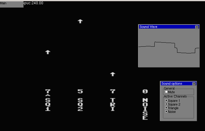
NES audio is composed of 4 signal components: 2 square waves, 1 triangle wave, and a noise channel. I remember when writing a NES emulator (back in University) that I was surprised at how the Super Mario Brothers song had used the noise channel as percussion.
So, given an input, we can do some Fourier analysis on the input (in block sizes of 1024, 2048, 4096 samples), and try to decompose the input audio signal into the best parameters from the NES signal components. Basically, I did this greedily, finding the best matching parameters (which are frequency, duty-cycle type, and volume) for each of the 4 waveforms. I guess harmonics should probably be handled better–and transients (like percussion) should likely be handled more effectively. Anway, it was fun to play around with this, and for the most part if you know how the audio is parameterized, you can easily simulate how things would sound.
But it is much more fulfilling to actually build a ROM. I noticed that there was a c-compiler (cc65) that already had support for NES, and that there was a runtime library with some crude drawing abilities. So the octave code, spits out a super inefficient c-code representation of the commands to drive the audio on the NES, and there is a small driver program to visualize some of the parameters of the audio channels.
It was fun debugging some issues in my emulator to get it to work with the ROM. Turns out the runtime library for cc65 was doing some self-modification of the code (for some tables or something) and my memory mappers weren’t handling that correctly (and ended up segfaulting). Anyway, the resulting interface looks like (the overlays are from my emulator):
The analysis code is here: https://github.com/nbirkbeck/nes-freq-audio
And there are some video examples, where hopefully you can make out the source song:
There are some cracks and pops, since the analysis code doesn’t try to maintain consistency of the waveform when switching parameters. I also tried to decompose the sound so that multiple NES machines could compose and make a more realistic rendering, but ultimately (I think due to synchronization) the result wasn’t worth posting.
Scrabble in a car…well almost
Every time I visit my folks at their cabin we end up playing some rounds of scrabble. We allow the use of some aids, e.g., online tools that help find all words that that consist of a set of letters. Since we usually drive up to visit them (usually takes about 16 hours, usually split across 2 days), I’m always looking for some toy problem to work on in the car. On the last trip back, I figured I would write a scrabble word placement helper that find the maximum move given the set of letters. I didn’t finish this on the last visit, but had a skeleton of the solver (but my lookup was slow).
This past Christmas, I decided to revive that project, and ended up with a much more clean and efficient implementation. It’s obviously a pain to input the status of a game without a user-interface, so I whipped up a quick barebones UI (and server) that allowed playing from the game from the start.
With that, it’s easy to pit a few of these optimal players against each other. They have no actual strategy, though, beyond trying to maximize the score that you could get with the letters on hand.
More info and details along with the code here: https://github.com/nbirkbeck/scrablve
Here’s an example of two of the auto-players playing against each other:
Playing around with Reinforcement Learning
While playing a video game (I believe Mafia 3, from previous Christmas, I believe), I had started to think about what a “fun” AI to play against would look like. I got excited about trying to spend some time learning a bit about this space, using a restricted/simpler game environment.
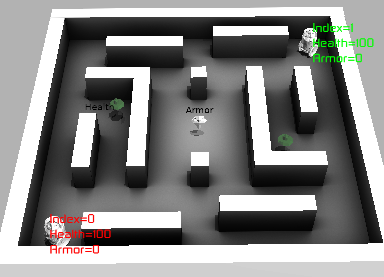
I decided that a simulation environment for a stripped down version of a 1st-person shooter game (mostly happening in 2D) would be sufficient. Agents can move around the environment and the objective is to shoot the opponent. The bullets look like little arrows and do a certain amount of damage (armor limits the damage).
Like Quake III (one of my all-time favorite games), there are some power-ups (health and armor). Controlling power-ups is necessary to be successful in this death-match game (first to hit a certain number of kills in a given time frame).
Simulation Libraries
The environment (world) and core actions of the agents are written in C++, where the agent gets observations from the world and returns a set of desired actions. Actions are carried out by the world, using proto-buffers for communication. This was mostly since I was designing this before thinking about how I would be interfacing with RL libraries.
In the end, I found that stable_baselines3 seemed like a reasonable RL python library, so I just had to adapt the python wrappers of the c++ core to expose what was necessary there.
So proto for data that needed to be serialized, bazel for build, gtest for testing (there aren’t many), stable baselines3 (for RL), and eventually Ogre and Blender cycles for rendering (see below).
Some example YouTube videos:
- Playing the game (1st person) against one of the agents: https://youtu.be/Dz061aS6qgM
- An example using the old (non-OGRE) rendering: https://youtu.be/h6Pw6QfVRgc
Code available: https://github.com/nbirkbeck/battle-ai
Agent Training using Reinforcement Learning
After a day or so of getting an environment ready, and then a bit more time integrating into an RL environment. I remember being slightly disappointed with the results. I think this was me being naive in terms of the amount of effort involved in tuning parameters / debugging models to get an agent to learn anything.
Finding power-ups
I had to dial things back to try to get an agent capable of even finding powerups. In that simpler environment, reward is proportional to the health or armor that the agent picks up, and actions are movement in one of 4 directions. Eventually, the agent did find a reasonable strategy to pick up items in a loop (but still missed finding one of the other health items that could have been more optimal). Likely, if I had better knowledge of the training algorithms / parameters / back-magic involved in tuning them, I could have found them.
Example: The agent starts out in the left of the video and does learn to pick up the health (middle left), and then go to the center (to get the armor). The agent then repeats this pattern.

There is also an example video here:: https://youtu.be/TCylBJaad6E
Higher-level actions
Seeing how long it took to get the agent to solve the simpler task of finding power-ups, and given I was interested in learning high-level strategies, I created the skeleton of a “plan-following” agent. This agent is parameterized in terms of behaviors (like go to a health or armor powerup, move towards the shortest path to a visible opponent, or move left, right, away from the opponent). The agent senses how far away from the items it is, as well as how far away from the opponent, it’s health/armor, etc.
I really wasn’t sure how to setup the parameters for the learning algorithms and just adapted them from other games (like the atari games). After several trials, I started adding more complexity in the rewards (e.g., reward for not standing still, for not hitting a wall, for getting health and powerups, as well as for killing the opponent, and negative reward for being killed). This just introduced more parameters that it wasn’t clear how to tune.
After some time of back-tracking my approach, just using a simple reward of “1” for killing the opponent seemed more desirable–given that really is all that matters in the end. After playing around with the training schedule and increasing the number of iterations, training loss was decreasing and the agent was doing better. Example: https://youtu.be/adXGj-8ppU0. But the agent still seemed “dumb”, e.g., it was avoiding going to nearby powerups when health was low. And the agent wasn’t better than the hard-coded agent I wrote in a few hours to bootstrap the training process (and to test out the planning).
After several more attempts, each training for about 1.5 days (20 Million steps) with various parameters, things weren’t getting significantly better. Ultimately, the best I got was by penalizing all of the left, right, forward, back actions in favor or just going for powerups. The agent could at least hold its own against the opponent it had been learning against:
Example video: https://www.youtube.com/watch?v=MYxv-7oNm38
In the end, during the process, I realized that my initial motivation to work on this problem was about a “fun” agent to play against. Training an agent to be good at the task was likely to not be a fun opponent to play against. I guess I got out of the project what I had intended, but like any other of these projects there are many fun digressions along the way.
Interesting Digressions
Either when training agents (and waiting for things to happen) or just looking for other things to clean-up before finalizing the project, there are always some interesting findings along the way.
Pyclif vs other wrappers
In previous projects (years ago), I had used Swig (http://www.swig.org) for creating python wrappers of my c++ code. And since I was using QT for many UI’s at the time, I ended up switching my personal libraries to SIP. I look fondly back on writing custom implementations for accessors with SIP as it gave some visibility on the raw python C API.
Another similar utility is CLIF (https://google.github.io/clif/), which I initially tried to use with this project. But for reasons that I can’t recall, I either couldn’t get it to work – or couldn’t get it working easily with Bazel (which was what I’d chosen to use for the build system).
However, in the process I came across Pybind (https://pybind11.readthedocs.io/en/stable/) as an alternative. And I ended up loving it. It is trivial to create the mappings, the code is all c++ (instead of a domain specific language), and the custom implementations (say for accessors) can be concisely written with lambdas in c++.
For example, I have an image class that I have been using for more than a decade that primarily uses operator overloading for accessors. When simply trying to export a heatmap for the examples above, dealing with the image libraries (e.g., PIL) for floating point RGB turned out to be painful to figure out in minutes. Since I already needed python wrappers for the Agent and World, it was easy enough to export the image interfaces, which were already being used in this project. Adding custom code (using set instead of operator) was easily accomplished with the following wrapper:
  py::class_(m, "Image8")
    .def(py::init<int, int, int>())
    .def("width", &Image8::getWidth)
    .def("height", &Image8::getHeight)
    .def("set", [](Image8& image, int x, int y, int c, int v) {
       image(x, y, c) = v;
    })
    .def("resize", &Image8::resize)
    .def("save", &Image8::save);
Blender Cycles Render For Ambient Occlusion
I really wanted to automate a somewhat decent rendering from a simple box-based specification of the world. Simple materials with ambient-occlusion in Blender seemed good enough, but the steps required to do it (and make sure it was synchronized with all the geometry) was a bit of a pain. Likely possible to whip some scripts up in blender directly, but since Blender was using Cycles under the hood maybe it was just as easy to use Cycles directly to bake in some ambient occlusion directly from the level specification.
Where things went wrong:
- I only ended up making one or two levels, so probably wouldn’t have been too much work to do this manually for those few cases
- After hacking up a simple visualization, I really didn’t want to get too distracted with graphics (or animations) – so I ended up searching for a rendering engine to use. I just decided to use Ogre, mostly because it was available and I’d heard of it before.
So the sequence of steps for creating a level is something like:
- Create the boxes in blender
- Export the proto representation of the world and a concatenated mesh representation
- Create the geometry and use cycles to do the ambient occlusion
- Load the geometry into blender so that it can be exported (and converted) to an appropriate Ogre form
Obviously, that could be simplified, but whatever.
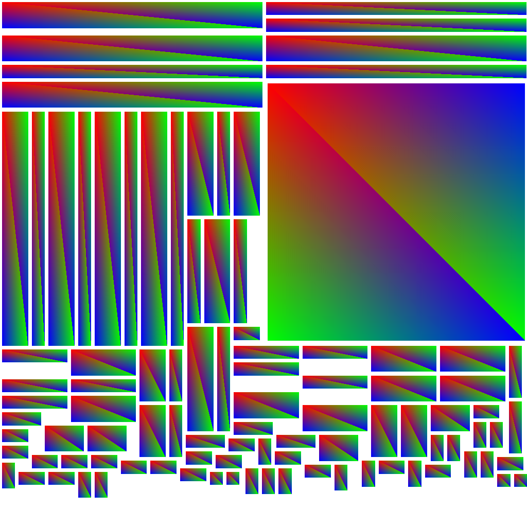
Resulting ambient occlusion map given below. With the example on the left being a handy trick I use all the time to rasterize barycentric coordinates of my triangles in the texture map.
Ogre for rendering
Some rough visualization was necessary, so I had just whipped up a quick visualization using some of the old libraries from my grad school days. But I still wanted it to look decent (hence the ambient occlusion digression), but when I was thinking about adding shadow, materials or animations, it seemed wasteful to do that without some other libraries.
I ended up using Ogre for this. Overall, this was a fairly painless transition, although I do remember the export and conversion of animations from blender to be a bit painful and required some time. Similarly for adding text.
Without ambient occlusion
Default interface (with ambient occlusion):
Ogre interface:
Checkout the videos instead:
- Ogre interface: https://youtu.be/MYxv-7oNm38
- Simple interface: https://youtu.be/h6Pw6QfVRgc
And with that, I think I’ve almost cleared my slate for this year’s christmas project (still TBD if at all…)
3D NES Emulator Renderer
A long time ago (sometime as an undergrad) I wrote a NES emulator (http://www.neilbirkbeck.com/?p=1054)
For some time, I’ve wanted to take either the rendered frames, or some game state and try to make a more appealing rendering of emulated games. I did finally get a chance to spend some time on this over the previous Christmas break. However, despite my best intentions of producing something that looked photo-realistic, it simply wasn’t practical to do in 4-5 days. I figure it is interesting enough to post what I ended up with here anyway.
The source code and some more details here (https://github.com/nbirkbeck/ennes). Although, the actual implementation depends on a bunch of my internal libraries (nimage, nmath, levset, and a bunch of other code from my PhD). At one point, I was tempted to use ideas similar to (http://www.neilbirkbeck.com/?p=1852) to try and get nice silhouettes for the upsampled images.
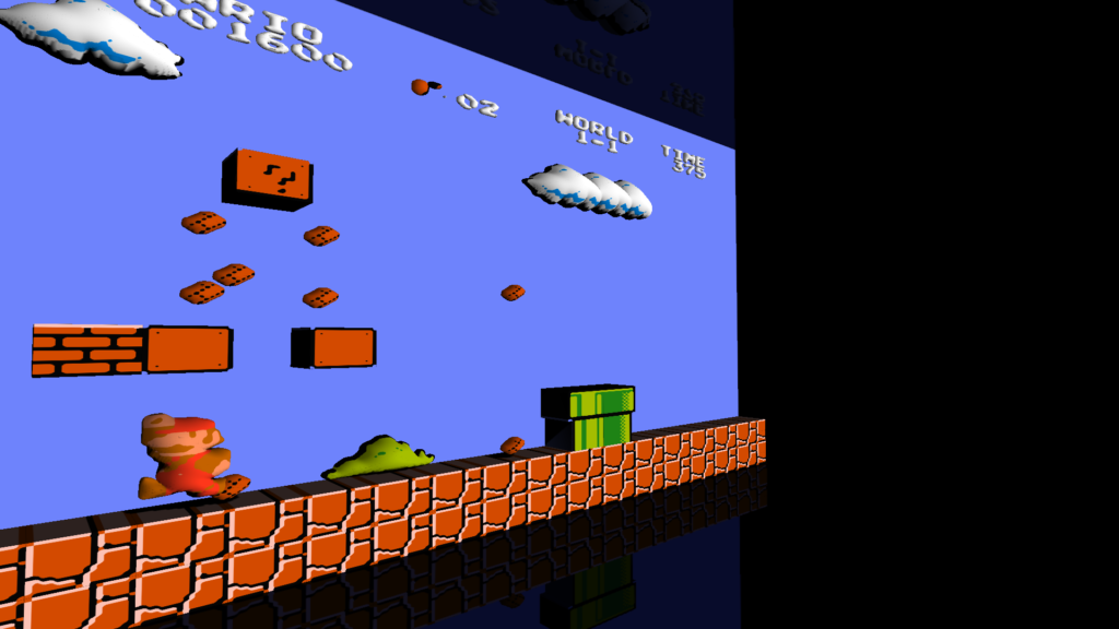
Here’s an example rendered video:
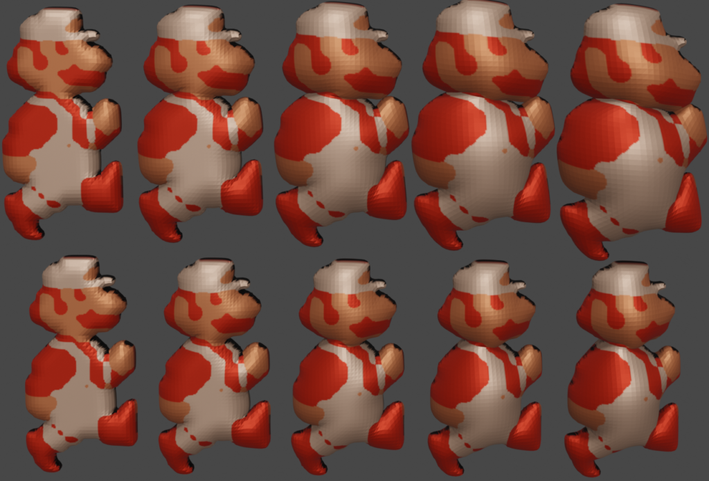
What I ended up doing was extracting the game state from the emulator, grouping sprites (based on colors), upsampling the images, producing a silhouette, and using those to extrude 3D geometries. For the most part, there is a cache that maps an sprite group to a corresponding 3D model. More details in the README.md on github. And there are a few hacks specific to super mario1 (which was mostly what I was thinking about when I started working on this).
Some examples of the puffed-up geometries:
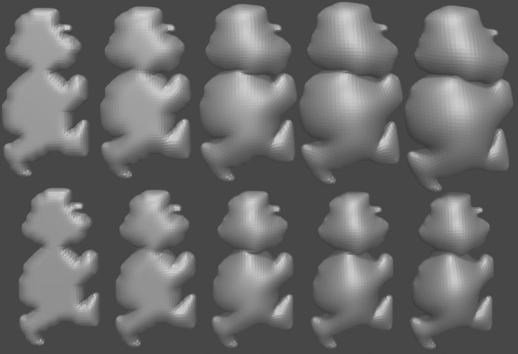
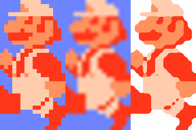
The following image (right) illustrates the upsampling used. (Left is nearest, and middle is image magick’s default)
And some screenshots (mostly from smb1):

One other noteworthy thing was just how bad the code was from the old emulator. For example, in rendering from the pattern table, there would be something like the following. And then there would be multiple versions of that code for the various options available for flipping the pattern (horizontally and vertically)
inline void drawByteBuf(int x,uint index,uint uppercolor,uint palette, int inc=1)
{
RGB_PE pe;
uint temp,temp2;
uint cindex;
uppercolor=(uppercolor<<2)|palette; temp = fetchMemory(&(g_ppu->memory),index);
temp2 = fetchMemory(&(g_ppu->memory),index+8);
cindex= ((temp>>7))| (0x2 & (temp2>>6));
if(cindex){
layer0[x]=uppercolor|cindex;
layer1[x]+=inc;
}
cindex= (0x1 &(temp>>6))| (0x2 & (temp2>>5));
if(cindex){
layer0[x+1]=uppercolor|cindex;
layer1[x+1]+=inc;
}
cindex= (0x1 &(temp>>5))| (0x2 & (temp2>>4));
if(cindex){
layer0[x+2]=uppercolor|cindex;
layer1[x+2]+=inc;
}
...
}
Contrast that to how simple a more comprehensive routine could be in the newer render_util.cc
Tetris on a plane
I’ve mentioned in a previous post that, that I’ve hacked up some quick versions of Tetris to pass time while travelling (see see this post).
I’ve had this other version kicking around, which I wrote after flying back from Europe on the train from San Francisco to San Jose. Its in an iframe below. Click on it and use (a,s,d,w)
Or open in a new window
Soko solve
Programming is a fun way to pass time.
A few years ago, I was playing lots of sokoban (or box pusher). Around the same time, I was also conducting a number of technical interviews, so was often thinking about self contained programming problems. Back as a grad student, in a single agent search class, we learned about searching with pattern databases–basically you solve an abstraction of the problem and use the solution length in that space to build up a heuristic (see this paper Additive Pattern Database Heuristics).
I’m sure there is plenty of research on the actual topic for sokoban, but I was interested in poking around the problem we were driving to Canada from California for a holiday.
The source code is up on github here:
https://github.com/nbirkbeck/soko-solve
And you can check out the demo (included in iframe below):
http://neilbirkbeck.com/soko-solve/
You can play the levels with ‘a’, ‘s’, ‘w’, ‘d’. Or you can click “solve” and “move” through the optimal path. The “Solve all” will benchmark a bunch of different methods. There is a much more detailed description of my analysis in these notes:
https://raw.githubusercontent.com/nbirkbeck/soko-solve/master/NOTES
Shape stylized images
Its been a very long time…
I realize that there are a bunch of side projects that are worth a short blog post. About 1.5 years ago, I was working on some coding tutorials to help a friend learn to program. One of starter projects we worked on was to generate a stylized image by populating an image with a bunch of dots (or other shapes). This is inspired by colorblindness test patterns, as I really wanted to generate a bunch of test patterns for testing video color characteristics that would easily allow you to determine if color metadata (e.g., primaries, matrix coefficients, transfer functions) were being interpreted correctly by a video processing system or display.
Well, I never did actually generate the actual test patterns with this code. But we did generate a couple of interesting images. Below are example Andre the Giant
 |
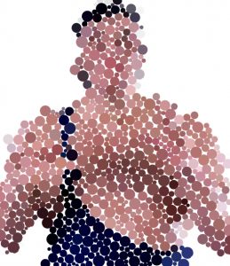 |
And here is another one that is a portrait of me:
Source code and sample input images on the github project: https://github.com/nbirkbeck/oneonetute
And a video:
JavaScript depth mesh renderer
Was playing around with some old code for generating depth maps and decided to create a demo that renders the depth maps in WebGL. The color video is stacked vertically on the depth texture so that the two will always be in sync. Looked into packing the depth into the 24-bit RGB channels, but as the video codec is using YUV there was significant loss and the depth looked horrible. A better approach would be to pack the data into the YUV channels, but I didn’t try. For this example, the depth is only 8-bit.
You can see the one video here:
http://js-depthmesh.appspot.com/
Stacked color and depth

Javascript & WebGL Image-based rendering demo
Back when I first started doing grad studies at the U of A, I worked with some others on image-based modeling and rendering (http://webdocs.cs.ualberta.ca/~vis/ibmr/rweb.php?target=main). Back then we had very specific renderers for the latest and greatest hardware (Keith Y. was the author of these), and I had worked a bit on a wxWidgets cross platform version of the renderer and the capture system.
The file format was a binary IFF-type format that could be used to stream partial models. Internally, look-up tables and texture basis images were represented either raw or in Jpeg. I originally just wanted to use emscripten to port that version to javascript, but kind of got discouraged after seeing some of the work that would have had to been done to the no-longer maintained renderer source, which had inline assembly and used ancient GL extensions, and I wasn’t sure what was required to interface with dependent libraries (like libz). Turns out you can natively do all of the necessary binary file unpacking (and jpeg/raw image decompression) to get things loaded into WebGL textures. Admittedly, some of these things are not as direct as they would be if you were calling say libjpeg to decompress, but interesting nonetheless. So here is a WebGL version of the renderer:
http://js-ibmr-renderer.appspot.com
that has almost all the same functionality as the desktop app (doesn’t do the 2D or cube-map look-up tables, and doesn’t support some of the older file formats). Should work with anything that has a decent graphics card and a browser that supports WebGL.
Source code: https://github.com/nbirkbeck/js-ibmr-renderer

Updated source files for the random shape generator
Updated some source files for the random shape generator:
http://www.neilbirkbeck.com/source/meldshape-0.1.zip
http://www.neilbirkbeck.com/source/tiling-0.1.zip
http://www.neilbirkbeck.com/source/rshape-0.2.zip
A voice basis
Not too long ago, Leslie and I were wondering about pronunciations of names. We had found a site that had some audio samples of the pronunciations, and we had started playing several of them over and over again. It sounded pretty funny listening to them, and I thought it would be neat to hear a real audio track represented with a bunch of people just saying names. Then you keep adding more people saying more different names until you get something that “sounds” like the input.
The set of audio samples of someone saying names, become a basis for your audio signal. I hacked together a quick program and some scripts to use a set of voices to represent an audio track. The algorithm simply tries to fit the audio samples to the input signal and keeps layering audio to fit the residual. It’s a greedy approach, where the best fit from the database is chosen first. Each layer positions as many database samples over the input signal (or residual signal) in a non-overlapping way (see the code for more details). There are probably much faster ways to dot his, perhaps using spectral techniques, but I wanted something quick and dirty (e.g., a few hours of work).
The result doesn’t sound near as compelling as I had imagined. To emphasize that it is just people speaking names that are used to produce the target audio track, I’ve broken the target audio track into 5 second segments. In the beginning, 5*pow(2, i) speakers are used to represent the signal for the i-th segment, so that the signal gets better as you listen longer.
The input audio track is a 60s sample from “Am I a Good Man”.
In the last segment, 10240 speakers are used to represent the signal. Results:
five_kmw.mp3:The best example as it has the most names and the most speakers (names that start with K, M, V)
five.mp3:uses fewer names (only those that start with K)
three.mp3. uses only 3*pow(2, i) voices at each segment, so the approximation is not as good.
Code (with scripts, in a zip file):audio_fit.zip
CameraCal
This is a camera calibration tool inspired by the toolbox for matlab. Give it a few checkerboard images, select some corners, and you get internal calibration parameters for your images.
Features:
- Output to xml/clb file
- Radial distortion
Windows binaries (source code) to come.
Updates, resume, cs-site, etc.
I guess this site will be undergoing an overhaul in the next little bit. Also, fixed up some issues with my CS pages (http://www.cs.ualberta.ca/~birkbeck)
I’m trying to get better at updating my resume (and the associated page on this site). In this regard, I’m grateful to my committee and graduate supervisors for my latest award (I’m just really slow posting this):
https://www.cs.ualberta.ca/research/awards-accolades/graduate
I’m honored to share this title with Amir-Massoud Farahmand.
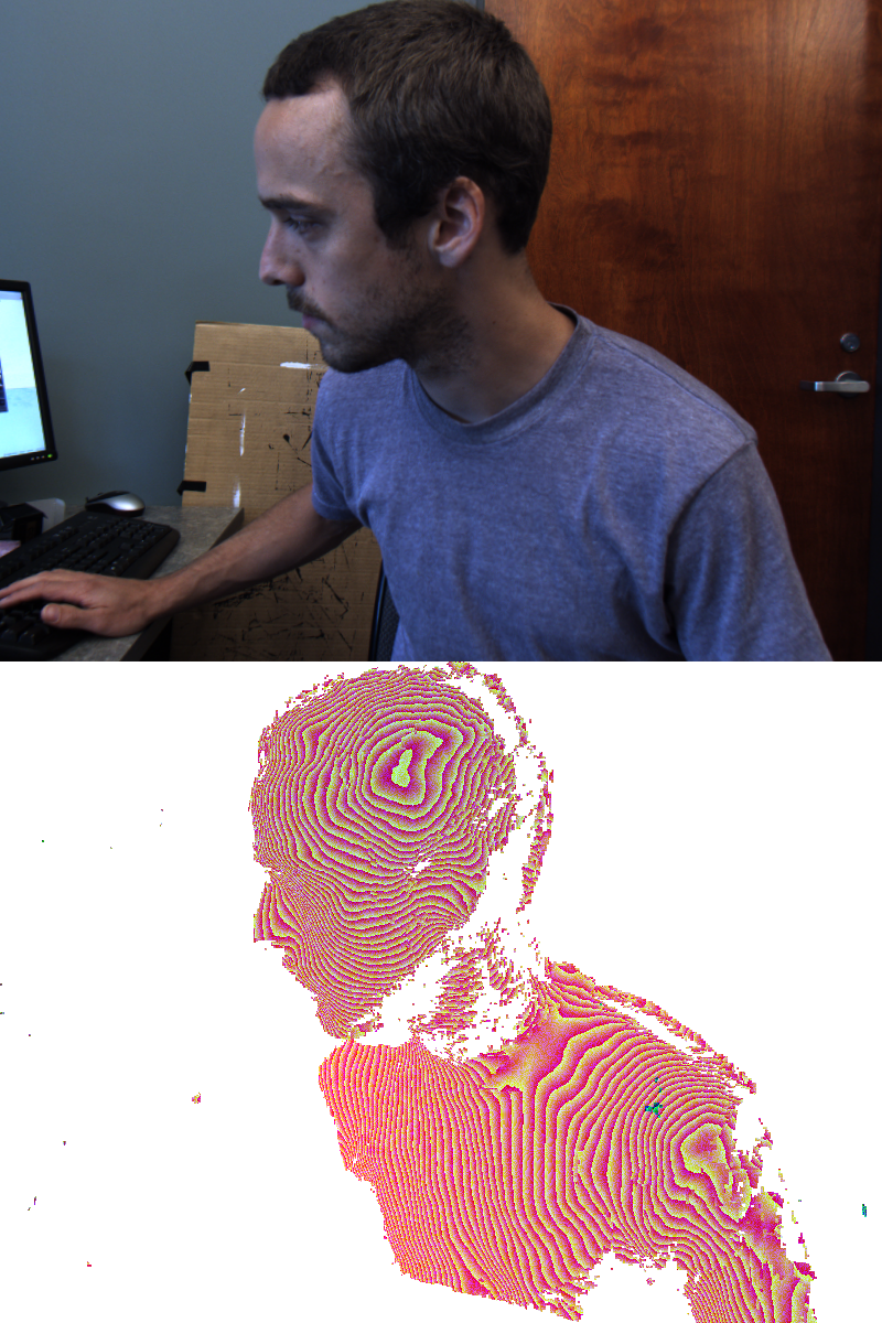
View-based texture transfer
I recently worked on a project where it was necessary to transfer a texture from an existing 3D source model to another similar target model. The target model shape is not exactly the same as the source model, and the topology and uv coordinates are different. While I am sure that there are likely specific methods for doing this (i.e., similar to how normal maps of higher resolution geometry are baked into a lower resolution texture). However, in this example, the geometry can be quite a bit different. In favor of using some existing tools that I have to solve this problem, I have a solution that is based on some of the work in my PhD on estimating texture of a 3D computer vision (CV) generated object when given calibrated images of the object (see section 4.4 , or this component). In CV, since the object geometry is estimated from images, it is only an approximation of the true geometry. For the problem of transferring a texture, we can use the same approach.
However, we are not given images of the source object, but we do have a texture so we can generate these synthetically. In this way, we can even give important views more weight (e.g., by having more views of say the front of the object). For the sake of illustration, I will demonstrate this on the teddy example (downloaded from www.blender-models.com). The source model has an accurate 3D geometry, and in this case the source model doesn’t have uv coordinates (the texture coordinates use the world coordinates for a volume-like texture, and the geometry encodes some detail). I have removed some of the detail on the eyes and nose, then the object has been decimated and smoothed so that its silhouette is quite a bit different than the original input geometry. The target object also has a set of non-optimal uv coordinates. The differences in the target object may make it difficult to simply find the corresponding point on the source object in order to transfer the texture (similar to what I’m guessing what would be used for the baking of normal maps).
 |
 |
 |
 |
| Teddy geometry (source) | Teddy wireframe (source) | Decimated (target) | Decimated wireframe (target) |
In order to transfer the texture from the source object to the target a number of synthetic images can be generated around the source object.
 |
 |
These images and the camera poses can be used as input to a texture reconstruction. In my PhD, I explored several alternatives for this problem. Among these is simply taking a weighted average (avg), computing an optimal view for each texel with some regularization (opt), and a multi-band weighting (multi). The last two can also be combined, so that the multi-band weight is used for low frequency and the high frequency info is grabbed from the optimal view. For the Teddy, I applied these methods to two configurations: a set of input images generated from the Teddy with illumination, and a set of images from the Teddy without illumination. For basic texture transfer the latter configuration would be used. After applying these to the Teddy, you can see that a weighted average is blurred due to the difference in the target from the source.
Lit images
 |
 |
 |
 |
 |
 |
 |
 |
 |
|
| Teddy input | Average | Opt | Multi | MultiOpt |
Unlit images
 |
 |
 |
 |
 |
| Teddy input | Average | Opt | Multi | MultiOpt |
The opt and multi both give excellent results despite the changes in the geometry, with some small artifacts (e.g., near the eyes for multi method). The combination of the two methods gives a good overall texture capable, fixing up some of the small artifacts. The opt method has some trouble with places that are not visible (e.g., under the chin). In my prototype implementation, I had some scripts to statically place the cameras and perform the rendering of the images in blender, but the cameras could be placed in order to get full coverage. The models and images are all available in the TeddyBlog.zip file.
Publications
Turns out I wasn’t very active updating the publications. It is now up to date (has things after 2008).
Its been a long time coming…
…not only for this post, but also the cleaning that I just started on the old filing cabinet. It feels nice to get rid of old paper, like receipts & visa statements, from over 10 years ago. The best part is going through the auto expenses, and basically discarding the entire folder–this last year with only one shared vehicle has been great.
One of the most painful folders to go through is the computer receipts. Its hard to swallow how much was spent on computer things. Back when I was just starting out as undergrad, I was playing a lot of Quake 3, and I got caught up in the “trying to have the latest hardware” cycle. This was also at a time when I was working a lot during the summer and still living with my folks, so maybe it was okay to spent $500 on the latest graphics card, if only to get a few more FPS out of quake.
Just out of curiousity I am going to tabulate all of the major expenses during that time:
Surprisingly, I only found receipts for a few mice and keyboards; they probably weren’t kept (Keyboards: 3, Mice: 4).
It all started somewhere around 1999, when I had just started university the year before. I remember upgrading our home computer for about $500, and was psyched that I could play DVDs on the TV with it. At about this time was when we first started to use the internet.
1999 ($253)
Quake 3 Arena Boxing Day ’99, $50
FaxModem $203
2000 ($3000!)
This was about the time when I really started to waste money upgrading and spending too much time playing quake. I think there was a time when I was upgrading our old computer from 133MHZ processors to slightly faster ones that I could find on the edm.forsale newsgroup. I was working two jobs over the summer and I had hurt myself skateboarding, so all of my efforts went into Q3. I can’t believe how much was spent, and I’m sure that I bought a huge 19 inch monitor for over $300 during this time. And these are only the ones I have receipts for. Many other things were purchased from individuals (and a few sold).
In my defense, I was helping build computers for my G/F at the time, and also for my parents, and brother (I think). The main problem is that I was caught up in the benchmarking scene. Its impossible to keep up with it. The other major cost associated with this was trying to overclock my Athlon. I had penciled in some marks on the chip to unlock the clock multiplier, and when putting the heatsink back down, I partially crushed the casing. A little later things weren’t working well (random blue screens), during quake, god forbid. I had to take it into two places: one charged me for more expensive ram, and the other found out that it was just that one of the cards wasn’t seated all that well. This chipped die went on to be a decent computer for years later.
Intel Pentium MMX-233 MHZ CPU $80
3DFX Voodoo3 2000 16MB $140
VooDoo3 300 16MB $115
13GB HDD $185
Thunderbird 800, $320
Asus A7V $250
Raid Controller $160
Tower $60
Samsung FDD $20
Power Surge $35
ASUS AGP V7700 GEFORE 2 GTS DELUXE 32MB $495
Gamepad: $55
Tower and 300 Watt PSU $80 + $45
Another diagonstic: $75
Diagnostic + 128 VCRAM: $295
CD writer: $339
Epson stylus: $250
2001 ($861)
Maybe I learnt my lesson from the previous year. 2001 didn’t seem so bad
Lexmark Printer: $246
HIS ATI Video Card $45
Speakers + SB Card $80 + $32
A7V133 Socket A, $188
MSI Starforce $145
Duron 750 $90
Duron Heatsink $35
2003 ($300)
ATI 9800 AGP128MB $300, April
2004 ($593):
Pyro video camera $80
Wireless router and card $183, 2004
Printer Ink and DVD writer: $330
2005 ($1024):
iPod Nano: $250
Samsung 17 inch monitor $387 * 2
2006 ($525):
LG Monitor $250,
160GB HD $90,
MSI 7600GS $185
Somewhere in between I bought Athlon 64 and kept that up until about 1.5 years ago.
It turns out that some of these things were actually good investments. Obviously graphics cards and printers are not. But the two monitors I bought in 2005 are still going strong. Same with the surge protector: don’t have to worry about the current T-storm we are having.
In the end, I’m glad I no longer try to keep up on the latest hardware, but at the time I guess it was exciting. It also seemed like things were changing faster back then.
Region-based tracking
I recently had to revisit some tracking from last year. In the process, I uncovered some other relevant works that were doing region-based tracking by essentially segmenting the image at the same time as registering a 3D object. The formulation is similar to Chan-Vese for image segmentation, however, instead of parameterizing the curve or region directly wiht a level-set, the segmentation is parameterized by the 3D pose parameters of a known 3D object. The pose parameters are then found by a gradient descent.
Surprisingly, the formulation is pretty simple. There are two similar derivations:
1) PWP3D: Real-time segmentation and racking of 3D objects, Prisacariu & Reid
2) S. Dambreville, R. Sandhu, A.Yezzi, and A. Tannenbaum. Robust 3D Pose Estimation and Efficient 2D Region-Based Segmentation from a 3D Shape Prior. In Proc. European Conf. on Computer Vision (ECCV), volume 5303, pages 169-182, 2008.
3) There is another one from 2007. Schamltz.
This is similar to aligning a shape to a known silhouette, but in this case the silhouette is estimated at the same time.
The versions are really similar, and I think the gradient in the two versions can be brought into agreement if you use the projected normal as an approximation to the gradient of the signed distance function (you then have to use the fact that = 0). This should actually benefit implementation 1) because you don’t need to compute the signed distance of the projected mesh.
I implemented the version (2), in what took maybe 1 hour late at night, and then a couple more hours of fiddling and testing it the next day. Version 1) claims real-time; my implementation isn’t real-time, but is probably on the order of a frame or 2 a second. The gradient descent seems quite dependent on the step size parameter, which IMO needs to change based on the scene context (size ot object, contrast between foreground and background).
Here are some of the results. In most of the examples, I used a 3D model of a duck. The beginning of the video illustrates that the method can track with a poor starting point. In fact, the geometry is also inaccurate (it comes from shape-from-silhouette, and has some artifacts on the bottom). In spite of this, the tracking is still pretty solid, although it seems more sensitive to rotation (not sure if this is just due to the parameterization).
Here are 4 videos illustrating the tracking (mostly on the same object). The last one is of a skinned geometry (probably could have gotten a better example, but it was late, and this was just for illustration anyhow).
http://www.youtube.com/watch?v=ffxXYGXEPOQ
http://www.youtube.com/watch?v=ygn5aY8L-wQ
http://www.youtube.com/watch?v=__3-QB_7jhM
http://www.youtube.com/watch?v=4lgemcZR87E
Linked-flow for long range correspondences
This last week, I thought I could use linked optic flow to obtain long range correspondences for part of my project. In fact, this simple method of linking pairwise flow works pretty well. The idea is to compute pairwise optic flow and link the tracks over time. Tracks that have too much forward-backward error (the method is similar to what is used in this paper, “Object segmentation by long term analysis of point trajectories”, Brox and Malik).
I didn’t end up using it for anything, but I wanted to at least put it up the web. In my implementation I used a grid to initialize the tracks and only kept tracks that had pairwise frame motion greater than a threshold, that were backward forward consistent (up to a threshold), and that were consistent for enough frames (increasing this threshold gives less tracks). New tracks can be added at any frame when there are no tracks close enough. The nice thing about this is that tracks can be added in texture-less region. In the end, the results are similar to what you would expect from the “Particle Video” method.
Here are a few screenshots on two scenes (rigid and non-rigid).

But it is better to look at the video:
Accordion Hero
Last weekend, I spent some time making a prototype Accordion Hero that uses live input from a microphone, does Fourier analysis to determine the keys, and uses this to control the video game. The beauty of this is that you can use your own instrument and try to learn while playing a game.
http://www.youtube.com/watch?v=dm4Kv_-Sen0
The version is just a prototype. While debugging the audio input, I used Audacity (which has a beautiful set of frequency analysis tools). These were helpful in determining if it was possible. I ended up using the tools for the spectral analysis from Audacity (they have an internal FFT that is pretty lightweight and saves linking to some other external library, e.g., fftw3). Also, the portaudio library is great for getting audio input across several platforms. I used it without a hitch for linux, mac, and cross-compiled windows. I’m a fan!
Common issues include a bit of lag, and some noticeable bugs where it says you played a note before you played it (this is actually a minor issue that is easy to resolve).
I spent some of today building the windows version:
AccordionHero.zip
the windows version has some problems (namely, it crashes on exit). Use the .bat script to run. It may be missing mingw.dll (should be easy to find on the web).
And a mac version:
AccordionHero-mac.zip
I am not sure I have packaged all of the dependencies. Again, run with the .sh file. You may have to use dylib-bundler (or the other mac tool to rename the libraries reference by the binary).
I didn’t spend much time tweaking for different systems. You will have to make sure that the audio level on your input is high enough. Use the ‘f’ key in the program to bring up the frequency spectrum. This should have a horizontal bar across it. This is the threshold, below which everything is ignored. Use the .bat/.sh script to adjust this file (the vertical scale is roughly -90 to 0, the default threshold is -65 DB).
I have only tested this with the Accordion, but it should work with other instruments. Use the ‘f’ key to find the frequencies of your instrument. Edit the notes.txt file (which serves as calibration).
Here are some screenshots of the very lame gameplay:


MeldShape

MeldShape is another application for generating random shapes. Although, unlike JShape, which produces shapes in an algorithmic way, MeldShape takes an initial set of shapes and evolves them using differential equations.
Each shape has a measure of speed over the domain, and tries to fill in the entire domain without conflicting with other shapes. There is also a measure of how much a shape can vary from its original shape. The evolution is performed using an implicit level-set implementation. More technical details: meldshape
Below there are binaries for both windows and Mac. The Mac version will require you to download a recent version of the open source Qt libraries. Open up the application, and drag a set of seed shapes from JShape onto the window. Use the evolve button to start the evolution.

The concept for this project was initiated for Mat Bushell.
Some movies of evolution:
And an unedited (poor quality) movie of how to use MeldShape in combination with JShape: meldshape-usage
Qt UiLoader runtime erros when cross-compiling
I was recently trying to build a windows version of the level-set shape generation (initial results, which is really a derivative of JShape), which is now titled MeldShape. The Mac version has come through several revisions now, and I figured if I was going to put anything up here, it might as well include everything (a document, some binaries, as well as a post).
Anyhow, I usually use a cross-compiler to build windows applications, and in the past I haven’t had any trouble getting a working build. However, this time was different.
I have working binaries for most of the libraries that MeldShape depends on, so building MeldShape was just a matter of updating these libraries and fixing any non-portable aspects within MeldShape. There were a few of these little things, like usleep and drand48, and checking validity of a pthread with (pthread_t*) != null (win32 pthread_t is a struct with a pointer inside). These things are obviously straightforward, and wouldn’t have even been an issue had I been thinking of a portable application in the first place. The real problem came within the Qt components.
When cross-compiling on linux for win32 targets, it is relatively straightforward to setup Qt. You use wine to install the windows libraries of Qt (the mingw build) and use your linux qmake with the appropriate spec file. Typically once you get the program to link you are out of the woods. But with Meldshape, linking was fine but running was always giving a symbol error in the Qt dll’s. It didn’t work either in Wine or in windows XP.
This was super frustrating, as I don’t have a working setup in windows using MinGW to build Qt applications. And in my experience, building in MinGW is really slow compared to the cross-compiler, so I really didn’t want to have to setup my environment from scratch (building from source). So I suffered through this problem, trying to figure out why on execution windows was complaining about missing symbols in the Dll (mostly in QtCore4.dll). I have seen similar problems to these when trying to run the executable with mismatched Dll’s (especially between the mingw and msvc builds of Qt), so I figured it had to be something with the versions of the Dll’s. I was using the same version as I had built with, so that was out.
I then tried an older version of Qt (since I had been using an older version in the past), and again no luck. With no other option, I started to strip my app to a barebones sample application to see if even that would work. And sure enough it was working fine (although it wasn’t referencing much else other than QApplication). The problem seemed to be something to do with one of the other libraries I was using.
I struggled with this for a while, and finally came up with the hypotheses that this was maybe due to loading parts of the UI with QUiLoader (from UiTools). After commenting out the few parts that use forms, it actually starts to work ???? This was at the point when I was ready to say, “screw the windows build”. I mean, the application is pretty simple, and at this point it is not even worth the effort. Anyway, I’m sure I am using forms in my other applications, so I have no idea at this point why using forms are causing problems with the Qt in windows. I decide to try QFormBuilder from the QtDesigner components instead. Luckily the API is pretty much the same, so almost no code (except for the declaration of the loader) has to change. Strangely enough, QFormBuilder worked fine.
I have no idea why QUiLoader was causing problems and QFormBuilder was not. I’m happy I found the problem, but at the same time I think the only reason I found it was due to luck. In the end it took almost 6 hours to find the problem and port the rest of the code…something I figured would take maybe 2 hours.
In the next little bit, I will try and upload the binaries and the technical document (as well as create a new project page for it)…all of the things that could have been done in that time it took to track down a non-sense bug.
1D peak detection with dynamic programming
Not too long ago, I was working on something where it was necessary to extract the correct locations of peaks in a 1D signal. The 1D input signal comes from some noisy measurement process, so some local method (e.g., thresholding) may not always produce the best results.
In our case, the underlying generator of the signal came from a process with a strong prior model. For simplicy, assume that the spacing between the peaks can be modeled as Gaussian with mean, mu, and standard deviation, sigma. Also, assuming that the input signal is the probability of a peak (e.g., the signal is real valued, in [0, 1]), the problem can be formulated in a more global way.
For example, in a Bayes approach, the problem would be formulated as maximizing p(model | signal), where the model = {x_1, x_2, …, x_k} is the set of points where the peaks occur in the signal. The MAP estimate is obtained by maximizing p(model | signal) ~= p(signal | model) p(model), or minimizing -log(p(signal | model)) – log(p(model)). Assuming a simple Gaussian distribution between the spacing of the peaks, the prior, p(model), is easily defined as \sum_{i=2}^N exp(((x_i – x_(i-1)) – mean)^2/(2 sigma)^2).
For the negative log-likelihood term, we can use something as simple as -log(p(signal | model)) = \sum_{x} signal(x) * f(x; model) + (1 – signal(x)) * (1 – f(x; model)). Where f(x; model) = 1 where for some j, x == x_j, and 0 otherwise.
On first encounter with this problem, it seemed like dynamic programming would be ideal to solve it. In order to use Dynamic programming, we relax the unknowns, x_i (represent the ordered locations of our peaks) and allow them to take on any value in the input domain. The dynamic programming solution is then straightforward. In the first pass, the total cost matrix for all the peak locations is created. For each variable x_i, we store for each possible input location, the total cost for that location and all previous variables. In order to compute the total cost for variable x_{i+1}, each possible input location finds the best combination of x_i’s total cost, the likelihood, and the prior cost between x_i and x_{i+1}.
The only difference is that at each peak location, the likelihood for the region after that peak location is not considered (until later) and the peak location is penalized for appearing before x_{i-1} (ensures ordering).
Once the total cost matrix, C, has been computed (e.g., NxM matrix with N peak locations and an input signal of length M), the likelihood beyond x_i can be considered. For each of the possible peak locations, we accumulate the likelihood beyond the candidate peak location (e.g., C(i, j) = sum(neg_log_likelihood(S(j+1: M))). If done this way, each row of the cost matrix now gives the total cost if we were to consider only i peaks in the input signal. That is, we get the best locations of the peaks for all possible numbers of peaks.
In the following synthetic examples, the global dynamic programming method was used to extract the peaks in the input signal, as well as the number of peaks present. The global method used searched for up to 5 more peaks than were present in the ground truth. For the top examples the input peaks had a mean of 14 and standard deviation of 2. The dynamic programming method used the ground truth from the underlying model during its prediction.
 Simple example, where a non global method would work |
 Another simple example, with more peaks, number automatically selected |
 A more difficult example with more noise (4 peaks) |
 A more difficult example with more noise (10 peaks) |
 A harder example, notice that the last peak is detected correctly, even though the input signal is almost homogeneous near it. |
 A harder example where it would be harder to select the ideal threshold. |
 The success of the global approach depends on the prior model providing some information in the presence of noise. With a small standard deviation, significant noise can be overcome (notice the high peak at around 70 in the input is not a true peak in the ground truth signal). |
 When the prior model has a large standard deviation, the global method can not as easily resolve ambiguities. In this case, the wrong number of peaks is selected and the peak near time 50 is missed. |
The above tables were generated in octave (dyprog1D source code).
Latest Movies


Random Movies