Not too long ago, I was working on something where it was necessary to extract the correct locations of peaks in a 1D signal. The 1D input signal comes from some noisy measurement process, so some local method (e.g., thresholding) may not always produce the best results.
In our case, the underlying generator of the signal came from a process with a strong prior model. For simplicy, assume that the spacing between the peaks can be modeled as Gaussian with mean, mu, and standard deviation, sigma. Also, assuming that the input signal is the probability of a peak (e.g., the signal is real valued, in [0, 1]), the problem can be formulated in a more global way.
For example, in a Bayes approach, the problem would be formulated as maximizing p(model | signal), where the model = {x_1, x_2, …, x_k} is the set of points where the peaks occur in the signal. The MAP estimate is obtained by maximizing p(model | signal) ~= p(signal | model) p(model), or minimizing -log(p(signal | model)) – log(p(model)). Assuming a simple Gaussian distribution between the spacing of the peaks, the prior, p(model), is easily defined as \sum_{i=2}^N exp(((x_i – x_(i-1)) – mean)^2/(2 sigma)^2).
For the negative log-likelihood term, we can use something as simple as -log(p(signal | model)) = \sum_{x} signal(x) * f(x; model) + (1 – signal(x)) * (1 – f(x; model)). Where f(x; model) = 1 where for some j, x == x_j, and 0 otherwise.
On first encounter with this problem, it seemed like dynamic programming would be ideal to solve it. In order to use Dynamic programming, we relax the unknowns, x_i (represent the ordered locations of our peaks) and allow them to take on any value in the input domain. The dynamic programming solution is then straightforward. In the first pass, the total cost matrix for all the peak locations is created. For each variable x_i, we store for each possible input location, the total cost for that location and all previous variables. In order to compute the total cost for variable x_{i+1}, each possible input location finds the best combination of x_i’s total cost, the likelihood, and the prior cost between x_i and x_{i+1}.
The only difference is that at each peak location, the likelihood for the region after that peak location is not considered (until later) and the peak location is penalized for appearing before x_{i-1} (ensures ordering).
Once the total cost matrix, C, has been computed (e.g., NxM matrix with N peak locations and an input signal of length M), the likelihood beyond x_i can be considered. For each of the possible peak locations, we accumulate the likelihood beyond the candidate peak location (e.g., C(i, j) = sum(neg_log_likelihood(S(j+1: M))). If done this way, each row of the cost matrix now gives the total cost if we were to consider only i peaks in the input signal. That is, we get the best locations of the peaks for all possible numbers of peaks.
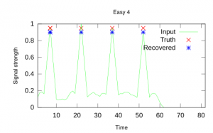
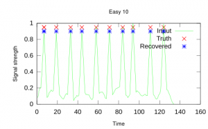
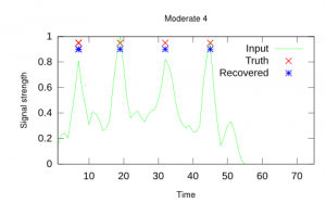
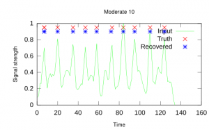
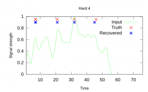
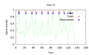
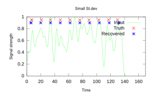
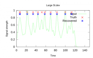
In the following synthetic examples, the global dynamic programming method was used to extract the peaks in the input signal, as well as the number of peaks present. The global method used searched for up to 5 more peaks than were present in the ground truth. For the top examples the input peaks had a mean of 14 and standard deviation of 2. The dynamic programming method used the ground truth from the underlying model during its prediction.
The above tables were generated in octave (dyprog1D source code).
