Archive for category Blog
Spectral regularization on computer vision problems?
I recently attended a talk by Robert Tibshirani, who mostly presented his work (and related developments) of the Lasso. The talk was very interesting, but I found some of his most recent work on spectral regularization for matrix completion particularly interesting. There are several problems in vision that suffer from unknown data, and this tool seemed like it could help out. I quickly prototyped some solutions using his/their approach and it does seem to have benefits in these applications, although I’m not sure of the impact.
I have written a draft document that details the problems that I was thinking about: spectral-reg-vision.pdf
And some quick and dirty matlab scripts that were used in the testing: spectreg
Using GPC
The polygon growing is coming along. Found this nice tool for polygon clipping: GPC. It is a C library that is all in one file. Nice and lightweight, efficient, and has a simple API (there are only a 6 or so functions, only two of which you need to use). And it does polygon union, difference, XOR, and something else I think. I’ve been using it to convery the meldshape (level set generated shapes) non-overlapping images (with spaces) into complete tilings of the plane:

Input (want to get rid of spaces)

Output (complete tiling, shapes do not overlap)
Maybe in the near future I will have the upload (it is a complement to JShape: the random shape generator). And also some details on how the GPC library was used to generate these.
GPU image registration code
Last year, at about this time, I went through an itch to implement various optic-flow algorithms. One that was brought to my attention by a classmate was the grid-powered non-linear registration from the medical community:
Shortly after implementing the method, I was driven to write a GPU optimized version. First, because I wanted to use Cuda. After I got started, I realized it was just as easy to implement the idea using shaders alone. I tested out using gauss-siedel to solve the sparse system of equations on the GPU needed for the diffusion component of the algorithm (they actually use adaptive operator splitting and a fast tri-diagonal solver in the paper, I believe). I remember not being all that impressed by the speedup that I attained (somewhat less than 2 times for this solver including read back, maybe 4 times without reading back). I ended up using an explicit filtering approach for the diffusion.
I wanted to post the code (it has some internal dependencies for creating windows and initing shaders, if anyone is interested I can supply): gpu-gauss-0.0.tar.gz
I didn’t actually compare the timings to the CPU implementation, but here is an example input sequence (same image perspectively warped):

Below is a cross-faded animation of the warped gifs. I didn’t really tweak the parameters (there are a couple for # iterations), but one-way flow took about 0.9 seconds on a geforce 8800 (including loading the images and saving, etc). This was run using the command: ./warp /tmp/w0.png /tmp/w1.png --seq=0 --its=20 --upd_its=20 --glob_its=40. There are a couple of artifacts around the boundary, but for the most part it looks pretty accurate. I have a couple other implementations of optic flow to post sometime.

Smooth depth proxies
Recently tested out an idea for using a view-dependent Laplacian smoothed depth for rendering. Given a set of 3D points and a camera viewpoint, the objective is to generate a dense surface for rendering. Could either do triangulation in 3D, in the image, or some other interpolation (or surface contouring).

This was a quick test of partitioning the image into bins and using the z-values of the projected points as constraints on a linear system with the Laplacian as smoothness. The result is a view-dependent depth that looks pretty good.
Check out the videos below. The videos show screenshots of two alternatives used for view-dependent texturing in a predictive display setting. Basically, an operator controls a robot (which has a camera on it). There is some delay in the robots response to the operators commands (mostly due to the velocity and acceleration constraints on the real robot). The operator, however, is presented with real-time feedback of the expected position of the camera. This is done by using the most recent geometry and projective texture mapping it with the most recent image. The videos show the real robot view (from PTAM in the foreground) and also the predicted view (that uses the geometric proxy) in the background. Notice the lag in the foreground image. The smooth surface has the a wireframe overlay of the bins used to compute the surface. It works pretty good.
- smooth-surface
- Or an alternative: tet-surface
Currently, the constraints are obtained from the average depth, although it may be more appropriate to use the min depth for the constraints. A slightly more detailed document is available (although it is pretty coarse): lapproxy.pdf
Another improvement would be to introduce some constraints over time (this could ensure that the motion of the surface over time is slow).
Level set shape generation
Not much to say about this yet. Trying to work on something for an artist. This is a first attempt. Starting from the same starting position, each of the other configurations have random stiffnesses, which means different images get generated.

Some movies:
Space-time texture used!
Again, we were recently working on a project involving a robot and a colleague’s (David Lovi’s) free space carving to acquire a coarse seen model. The model is fine as a proxy for view-dependent texturing (e.g., lab-flythrough):
But to generate a figure it is nice to have a single texture map. Since the geometry is course, a simple averaging is out of the question:
 After some minor updates to my initial implementation (to take into account the fact that all images were inside the model), the space-time texture map (idea anyhow) seems to work pretty good. Remember that this assigns a single image to each triangle, but it does so in a manner that tries to assign neighboring triangles values that agree with one another while ensuring that the triangle projects to a large area in the chosen image.
 Of course the texture coordinates above are not the greatest. The texture was generated from some 60 keyframes. The vantage points below give you an idea of the quality of the texture:

Again, the model is coarse (obtained from key-points and carving), but space-time texture map idea works pretty good to get a single texture.
The data for the model was obtained with the prototype system (described in this video http://www.neilbirkbeck.com/wp/wp-content/uploads/2010/03/IROS_predisp.mp4)
Interrupted trapezoidal velocity profile.
We were recently working with the WAM robot and needed to generate trajectories from a haptic device. The WAM code-base had code for following a simple trapezoidal trajectory. It is straightforward to generate such a trajectory given
maximum velocity and acceleration constraints.

Trapezoid velocity profile
The WAM library routines allowed to issue more positional commands (using MoveWAM), but the previous trajectory would be halted and the new one started with an initial velocity of zero. The figure below illustrates what would happen:
Clearly the p(t) curve is not smooth at the time of the new interruption (v(t) is discontinuous); this is evident in the robot motion. A worse case occurs when the commands are issued more frequently, implying that the trajectory can never reach
full velocity.

Trapezoid interrupt
Instead of creating a new trajectory with zero velocity, especially when the subsequent commands are the same as the previous command, the trajectory should take into account the current velocity. So instead of the result above, the interruption should still
produce a curve more like that in the first figure. Regardless of where the interrupted commadn is received (or its location), the resulting positional trajectory should obey the constriants. For example:

The implementation is straightfoward. There are main two cases to handle. Like before, if the distance to travel is large, the trajectory will have a period owhere the velocity is at maximum velocity. The details of the implementation are in the attached document (trapezoid-writeup)
Results
The figures below illustrate what the curves look like (red always starts at zero velocity, and white utilize current velocity).

Sample trapezoid trajectory.

The bottom figure illustrates the non-smoothness of the trajectories that would be generated if the current velocity is ignored.
Video
trap.mov
See it in action here: IROS_predisp
Python Code
A quick python prototype was used to validate the first step. Click on the window at the y-location you want the curve to go to. Currently the implementation actually uses the velocity profile and needs to integrate (uses simple Euler method to do so). Alternatively, you could easily store the positional curve and just look up the position.
rob.py
Direct multi-camera tracking with multiple cameras and Jacobian factorization?
I recently read the paper entitled A direct approach for efficiently tracking with 3D Morphable Models by Muoz et al (published in ICCV 2009). I was curious whether their technique for pre-computing some of the derivatives could extend to both multiple cameras and to a skinned mesh (as opposed to a set of basis deformations). I spent a couple days understanding, implementing, and trying to extend this idea. This blog and accompanying document is a summary of my results and relies heavily on the ideas in that paper. The pdf document, rigidtrack2 ,contains my thoughts (roughly). Most of them are concerns about speed, gradient equivalency, etc.
Here are some videos of the tracking (the left/top uses a an image-based Jacobian), and the right uses Jacobian computed in the texture space with factorization. The pose of the object in the middle is being inferred from the surrounding images. Notice that the bottom/right video has a mistrack.
Links to the other videos are here:
Those prefixed with “fact” use factorized; those prefixed with image use the non-factorized image Jacobian. The suffix is how many of the images are used.
The factorized Jacobian seems to perform worse, and is slightly slower, but this may be due to implementation error. It loses track in this example sequence (which has either four or one cameras), mostly due to the fast motion.
I have also uploaded the code: rigid-tracker-src.tar. It is kind of a mess, and won’t compile unless you have some of my other libraries. Check the TODO to see any limitations. But it may be useful if someone is considering implementing the same paper.
The blender sequences, .obj, and png files: RigidTrack2.tar
X-
I have recently fallen for boost::serialization. Super useful. Beats making your own file format, and you get serialization of stl containers for free. The newly added boost::property_tree also seems like it will come in handy.
The holidays are just about over. This last weekend was pretty fun. We went for a 13KM x-country ski (which, due to our lacking technique, just about killed us). The only thing that kept me going through the last bit was the the thought of the ravioli we were going to hand-make afterwards. It turned out pretty damn good. The dough was a little thick on the first couple batches (evidenced by the fact that the recipe was supposed to make 150 ravioli and we only got like 48 out of it). For future reference, we used the recipe from http://www.ravioliroller.com/recipes/basic.html.
And we went for a short shred today (at valley of all places). This lasted all of 1.5 hrs, but was fun nonetheless.
Finally finished up the vertmat blog. Check it http://www.neilbirkbeck.com/?p=1652. Still have to fix up some things, and possibly rebuild the binaries. I have to return the book that helped understand the derivation of the stress matrix, again for a personal note, it is the book cited by the IVM paper: Finite Element Modeling for Stress Analysis, by Robert Cook. All that was needed from this was the understanding of the strains (and how they are used with the linear strain tetrahedron). The strains are the partial derivatives of the displacements w.r.t x, y, and z (along with three mixed derivatives). As the displacements are interpolated over the triangles, I derived these from the barycentric coordinates of a point in the triangle.
Space-time texture map
There was a paper in 3DIM’09 entitled something like space-time consistent texture maps. The paper talks about how to construct a single consistent texture map from a multi-view video sequence of a moving subject. The method assumes as input a consistent triangular mesh (over all time sequences) and the input images. The problem is posed as a labelling problem: for each triangle compute the view (and time step) from which to sample its texture.
This framework obviously holds for the capture of static objects (where the number of labels is just equal to the number of images). This optimization framework is an alternative to other approaches, such as the naive solution of just averaging textures using all image observations. Such simple averaging does not work if the geometry is inaccurate (see image to the right of the blurry house, mostly on the side). I was curious if such a labelling approach would work better on approximate geometries, or whether it could be extended to a view-dependent formulation.
In the original formulation, the data term for a triangle in a view takes into account how much area is covered by the projected triangle (e.g., it prefers to assign a triangle to a view where it’s projected area is large). The smoothness term then takes into account the color differences along an edge. In other words if two triangles are labelled differently, then a labelling that has similar colors along the edge should be preferred. This problem can then be solved (approximately) with graph-cuts using alpha-expansions.
The last couple nights, for some reason, I kept having this thought that this same framework could be used to estimate some sort of view-dependent texture map (where instead of just finding the single best texture, you find several (say 4) texture maps that will work best in a view-dependent case). All that would need to be changed is the data term, and then incorporate some notion of view-dependent consistency (e.g., instead of just using the color difference on edges in the texture maps for neighbouring triangles, a similar cost could be measured on the edges after rendering from several views).
Basic implementation
I started implementing the basic framework. Below are some example results. Although, the method should really work best when used with accurate geometry, I wanted to test out the method when the geometry was only approximately known. In this sequence, the house is reconstructed using shape-from-silhouette, meaning that the concavities beside the chimney are not in the reconstructed geometry. Again, the image at the beginning of the blog (and at the right) show the results of simply averaging input images in the texture.
The left-most image shows the results with no smoothing (e.g., the best front-facing image is chosen for each triangle, followed by the solution using increasing smoothness weightings). There are some artefacts, especially on the left hand side of the house (by the chimney, where the geometry is incorrect). Increasing the smoothness helps out a bit, but too much smoothness samples the side regions of the texture from the front-facing images (which makes the blurry). See the movie to get a better idea of the problems.

Reconstructed textures for the house (left no smooth, right two increasing smoothness).
The texture maps for no smooth (best front-face image), smoothness=1, and smoothness=2, are given below. The gray-scale images show which input image the texture was assigned from (notice that the leftmost is patchy, where the right image suggests that large regions sampled texture from the same input image).
 |
 |
 |
 |
 |
 |
Dog results
I also tried this for a model where the geometry was much more accurate (the dog). It is hard to actually see any artefacts with the naive approach of just sampling the best view for each triangle (left-most image below).

Again, below are the corresponding texture maps and the gray-scale images denoting where the texture was sampled from. Again, increasing the smoothness definitely reduces the number of small pieces ni the texture. But it is hard to actually see any visually difference on the results. Check the video to see for yourself.
 |
 |
 |
 |
 |
 |
It is much easier to visualize the textures on the object. The blender models and reconstructed textures are uploaded if you want to check them out: models & textures.
View-dependent extensions
Shortly after implementing this, and before starting on the view-dependent extensions, I realized that I was going to run into some problems with the discrete labelling. If you have n images and you want to find a set of 4 view-dependent texture maps, you will need n choose 4 labels. Even with as few as 20 input images, this gives 4845 labels. After running into this problem, I didn’t further formalize the enery for the view-dependent case.
Iterative mesh deformation tracking

Patches on mesh (left) and a different target mesh
Another idea that interested me from ICCV (or 3DIM actually) was related to tracking deforming geometry, using only raw geometry no color. The paper in particular ( Iterative Mesh Deformation for Dense Surface Tracking, Cagniart et al.) didn’t require even geometric feature extraction, but rather relied on a non-rigid deformation scheme that was similar to iterated closest points (ICP). The only assumption is an input geometry that has the same topology of what you would like to track. As for the ICP component, instead of doing this for the entire model, the target mesh contributes a displacement (proportional to cosine between normals) to its closest vertex on the deforming source mesh. The source mesh is then partitioned into a set of patches, and each patch tries to compute a transformation that satisfies the point-wise constraints. The positional constraint on the patch center is then used in a Laplacian (or more specifically, the As-Rigid-As-Possible (ARAP) Surface deformation framework) to deform the geometry. This is then iterated, and a new partitioning is used at each frame. To ensure some more rigidity of the model, the positional constraint on the patch center is influenced by it’s neighboring patches, as well as by the transformation of the original source mesh. Look at the paper for full details.
I needed the ARAP for some other project (see previous blog), and decided to go ahead and try to implement this (I think it was actually last Friday that I was playing around with it). Anyhow, this week I knew that I had to test it on some more realistic data; my first tests were of tracking perturbations of the same geometry (or of a deforming geometry with the same topology). To generate some synthetic data, I rendered 14 viewpoints of a synthetic human subject performing a walking motion (the motion is actually a drunk walk from the CMU motion capture database). For each time frame, I computed the visual hull and used the initial geometry to try and track the deforming geometry. This gives a consistent cross-parameterization of the meshes over the entire sequence.
After tweaking some of the parameters (e.g., the number of iterations, and the amount of rigidity, the number of patches), I was able to get some decent results. See some of the attached videos.
Links to movies (if the above didn’t work):
Source blender file (to create the sequence, some of the scripts I use often are in the text file): person-final-small
Elk island motion
Two weekends ago we went to Elk Island. I’m not sure how it started, but we took a bunch of jumping pictures. And then tried to create some crappy stop-motion. As facebook didn’t like animated GIF’s, I uploaded the images here, and didn’t realize they had no corresponding blog. So here it is. You will have to click on the images to view the animation (it got lost in the downsample).


Trouble with generating synthetic wrinkle data from real-images
About mid September I wanted to create a synthetic data-set of wrinkle motion from real data. The synthetic data set had some constraints, such that the motion should be smooth and the cloth should not be too loose and wavy. I figured that I would just capture a sequence of real deforming clothing and then map a mesh onto the motion of the data. I realized that I was going to have to write some code to do this (and I also wasn’t afraid to specify plenty of manual correspondences). The input sequence looked roughly like below (captured from 4 cameras).

Input sequence for synthetic data (view 1 of 4)


The initial flat model (top) and enlarged model (bottom)
I figured I would use a combination of user (and by user I mean me) constraints and possibly photometric information (e.g., silhouettes, and image intensities) to align a template model to the images. But first, I needed a template model. For this, I captured a front and back view of the shirt I was wearing, and created a flat polygonal model by clicking on the boundaries of the shirt in Blender. In this way it is straightforward to get a distortion free uv-parameters. The next step was to create a bulged model. It turns out some of the garment capture literature already does something similar. The technique is based on blowing up the model in the normal direction, while ensuring that the faces do not stretch (or compress) too much. The details of avoiding stretch are given by the interactive plush design tool Plushie.
As for mapping this model to the images, I had previously written some code to manaully make models from images (by clicking on corresponding points in multiple images). I figured that something like this would be sufficient for aligning the template model. In the UI, you click on points in multiple images, and the corresponding 3D point is triangulated. These points are then associated with the corresponding point on the mesh (again manually). Finally, some optimization that minimizes deformation of the clothing and fits the points would be necessary. Originally, my intentions were to just try this for a couple frames individually, and later try to do some temporal refinement.
For the optimization, my first thought was just to use the Laplacian mesh deformation framework, but a naive implementation is rotational variant and doesn’t work well. After ICCV I noticed that the “As rigid as possible deformation” framework (which is similar to the Laplacian coordinates) would work perfect for this. I plugged in the code, and quickly realized that I was going to need a large number of constraints, more than I had originally thought would be necessary.
One of the biggest problems was that when I wore the shirt the arm top of the template model did not necessarily match the top of my arm, meaning that parts of the template model that were frontfacing in the template were not observed. This means that there was no easy way to constrain them to be behind (I only had camera views of the front). Some silhouette constraints would help this problem. The other problem (which may be due to the shirt) was that it is really hard to determine correspondences between the input and the mesh when the sleeve has twisted. I think I have to give up on this approach for now. I am considering using either animated cloth data (which in Blender seems to be too dynamic, and doesn’t exhibit wrinkles). Another method may be to manually introduce wrinkles into a synthetic model (I have just finished reading some papers on this and have a couple of ideas). The third method would be to use some color coded pattern to automatically obtain dense correspondences (e.g., google “garment motion capture using color-coded patterns”, or go here)
The last one is obviously too much work for what I actually want to do with it, but it is tempting.


Clicking interface (left) and initial/mapped model (right)


View-dependent texture mapping, shows that the areas with constraints are pretty good. But the other regions aren’t even close. You can also see how much of the front of the shirt on the template is actually not visible. Without constraint, the ARAP deformation puts it on front
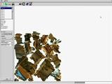
Image operation (shear/block/edge)
I got this idea for a cool image operation from an image in the book “Conceptual Blockbusting”. The seed image was basically just a bunch of sheared black and white rectangles. I wanted to create a similar image from some source image, but have a bunch of colored rectangles. I ended up using rotated and scaled rectangles. The result wasn’t near as good as I had hoped, but I figured since I wasted a little bit of time on it, that it was worth sharing. I tried adding edges as well. Didn’t work out all that great but whatever.
Check out the source code. It requires some code from a previous post on shock filtering, and it uses cairo to do the drawing (shear source code).


return ICCV – 09;
I found this old blog on my Destkop (it is about a week dated, but I wanted to post it so I can delete the file).
The quality of the papers at ICCV 2009 is amazing! This morning there were a couple talks on geometry that were especially interesting to me. One of them brings together much of the research in the last several years to allow efficient distributed reconstruction of city size scenes from unordered photo collections (Reconstructing Rome in a Day).
Yasu Furukawa’s recent reconstruction results are also very impressive.
The Microsoft research group never ceases to impress.
As promised
Here it is. Gimp coherence enhancing shock filtering. Install gimp and the related developer tools and build the plug-in (update: I was able to cross-compile it gimp-shocker.exe). Let me know if it works. This is a preliminary version.
Source code:gimp-shock.tar.gz

Moustache (Input)


Code Complete
I recently finished reading Steve McConnell’s “Code Complete”. In hindsight, I should have kept a list of all of the great things contained inside the book. The book is packed with information on software design and construction, lots of examples, and even more references to other sources. McConnell outlines the professional development plan used at his company, making it easy for anyone to get on a useful reading track.
And I have. I have read two of the references within this book (not necessarily in the professional development plan), and they have turned out to be worthwhile. The first was a classic, “How to win friends & influence people”, b Dale Carnegie. The other was, Conceptual Blockbusting.
Another related Amazon suggested reading was Donald Norman’s, “The design of everyday things”. I read most of this on my plane ride to Japan, and finished it this morning. It talks about all the things designers should (and shouldn’t do) to make products (or software) easy, intuitive, and just plain user-friendly. The book is comforting in the sense that it discusses how failure to use something (a tool, a software), is often the fault of bad design. Out of the book, some of the most important points of design are really what should be almost common sense; things like providing a clear mental model, making the system state visible, hiding functions that aren’t necessary for a task, and using standards. The book gives plenty of good references to everyday objects that were poorly designed (several examples of doors and faucets). And I was even surprised to read that the author uses (or used) emacs. I will definitely be coming back to this book the next time I (try) and design a UI.
Papercut
Well, I was on my way to Japan this morning (I guess it was technically yesterday morning), and I had recently cut my finger putting away some dishes into a picnic basket. While waiting in line, I asked a man behind me in line for his pen, and realized when I was using his pen that my finger was bleeding all over the page that I was trying to fill in. I don’t think that he noticed, but I am sure that he wouldn’t have been too happy about a stranger bleeding all over his pen. No big deal; what he doesn’t know can’t hurt him. Besides, I’m pretty sure that the blood donor clinic would have let me know if I had some serious disease (I visited them last month and haven’t been into any risky activity since then).
Anyhow, I continue onto customs and fill out the redundant custom form. Again, noting that my finger is kind of bleeding, but at least thinking that it was contained. As I got up to the customs guard, I dropped some blood on his counter and quickly tried to wipe it off. I looked down and noticed that there was some on the form that I had just finished completing. “Are you bleeding he says”, looking over to the counter where I left a droplet. I confirmed, and he half-assed put on some gloves, cleaned up the counter, and said that it was hazardous or something. I was thinking that I was going to miss my flight because my finger is barely bleeding–the cut is almost as minor as a paper cut. But he just escorted me to some other guards that gave me a band-aid and some hand sanitizer.
He was pretty nice about it, but I am sure that it ruined his day. If the tables were turned, and if I were at a certain paranoid phase in my life, I would probably have anticipated the worst (maybe even years later). Anyhow, if you are reading this, I am sorry. There were no band-aids at our house, and this was not top priority at 3:30AM when gathering my shit to go overseas.
Actually, come to think of it. For how often I have had open wounds, in some dirty places (e.g., skate spots covered in pigeon shit), I am surprised that I am not more concerned about thinks like this.
OpenOffice3
Wow! OpenOffice3 rules. But it reaches its true potential only when gstreamer is used as the backend for video. I am sure that I have run into this problem before: make a presentation on one platform (some fedora core). and then go to transfer to another computer and decide to upgrade OpenOfffice. I would typically do this using the binaries from OpenOffice, and then fiddle around with settings wondering why my ffmpeg encoded videos no longer work. The problem is that the binary packages on OpenOffice’s site are not packaged with the gstreamer back-end. For sure the version in fedora’s repositories use gstreamer.
In order to get this working last night, I decided to just upgrade to FC11 on my laptop. This was rather painless, and most of my own code compiled without problems. It seems that they are still cleaning up the standard include files, so I just had to add some missing “#include
Japan tomorrow. And I am friggin’ tired.
OOoLatex
I’m always on the fence about what to use for creating presentations. Whenever there are formulas (and you have already written a paper) it is nice to use the pdf/latex tools for presentations. But then again, laying out the images and embedding movies in these presentations nearly outweighs any benefits.
On the other hand, it is nice to have the layout (& movie) features of OpenOffice, but it would have been nice if OpenOffice used latex natively for its formula editor. Enter OOolatex, the latex editor extension for OpenOffice. This is a duo that is hard to beat.
Tobogganing image effects
Not too long ago I was reading a bunch of segmentation papers and came across “tobogganing” for unsupervised hierarchical image segmentation/clustering. Tobogganing is similar to watersheds and starts by clustering pixels into neighboring pixels that have the lowest gradient magnitude. The technique is efficient and can be made hierarchical by introducing a measure of similarity between neighboring clusters (the similarity is based on average colors and variances). This gives rise to a hierarchy of segmentations.
The method was used in LiveWire-based segmentation techniques (i.e., intelligent scissors), and has also been used in its hierarchical form for interactive medical image segmentation. In the latter application, the
hierarchy allows for quick solutions by computing the solution on the coarsest levels, and only refining it to finer levels when necessary. Thus avoiding redundant computation far away from the segmentation boundary.
I was interested in this application of tobogganing, and had to refrain from trying to implement it as I had no real use for it. But I also thought that the method might be useful for creating interesting image effects, which would be useful in another side-project. So, with application in mind, I tried a quick implementation this past weekend.
I have several potential ways of using the segmentation, but one of them was to try and help identify image edges that were more salient than the ones you typically get out of an edge processing algorithm (maybe smoothing regions with some Laplacian regularizer would give neat looking shading).
Below are some illustrations of the hierarchy for some input images. Tobogganed regions have been replaced with their average color.

Tobogganing effects (bike image)

Les neil tobogganing segmentation
The rightmost image gives an idea of how image edges could be used; the image edges extracted from an edge operator have been modulated with those extracted from the coarse levels of the tobogganed regions. Click on image for full-resolution. They are pretty big.
Preliminary source code:
iPhone sqlite3 slow joins?
A friend and I have been working on a small iPhone app, and we have been using an sql database for our data store. There had been large lags in our system for loading/saving (which we have now made lazy), but the majority of this was due to encoding images as PNGs/JPEGs. The storing into BLOBs didn’t appear to be all that slow, so I am fairly confident that sqlite3 was not to blame.
However, in our initial UITableView a number of objects are loaded from the database, and contain thumbnails (64×64 ish), and some meta-data collected from a simple join on a couple tables. This join collected information from children objects (such as size of blobs), and number of children objects. Surprisingly, with only 8 objects in the database, this loading step sometimes took longer than 2 seconds (including DB setup time). This timing seemed to scale roughly linear with the number of objects in the DB.
| Num Objects | Using join | Cached stats |
| 3 | 0.95 | 0.53 |
| 5 | 1.12 | 0.65 |
| 7 | 1.33 | 0.81 |
| 8 | 1.44 | 0.84 |
So each entry adds roughly 0.11s, and initialization takes roughly 0.4-0.5s. We get a slight improvement with caching the sizes (again I find this odd, as there are so few entries in the DB). Taking out the processing for the thumbnails (decoding), the times for 3 entries drop from 0.95 to 0.55 and 0.53 to 0.16 (for cached). So loading 4 thumbnails takes roughly 0.4/3s, approx 0.13s. This still seems pretty slow, but the difference in 0.55 and 0.16 seems to suggest that the originial query is that much slower.
I still think that this loading should be faster, but we may have to look into other ways to load the header info if there are many entries.
Long time, no bloody post.
Sometime, about two weeks ago, I decided to give blood for the first time. This is one of those things that I have wanted to do for a long time, but for some reason never got around to making an appointment.
After making the appointment, I was anticipating the donation. I figure I am a pretty healthy guy, and went in to my appointment about an hour after eating a hearty meal of veggie nuggets and heaps of pasta. I haven’t been drinking coffee lately, but I figured I drank as much water as I normally would (which really isn’t all that much). After being hooked up to the passive blood-sucking machine, I enjoyed watching my body’s red-oil drain out. After all, it is for a good cause; unlike fossil fuels, it is renewable.
The donation tech had mentioned to let her know if I started to feel strange. Sure enough, somewhere halfway in, I started to feel strange. I waited just long enough so that I could barely express this feeling to the tech, and within seconds they had me propped up in the seat with moist towelettes on my forehead. I was within seconds of passing out; the transfusion was stopped. I had never felt this before, and remained in a state of half awareness while contemplating what had just happened. Slightly embarrassed that I wasn’t able to donate blood properly. Naturally, I started to question if there was something that I could have done differently.
I could have drank more water. And maybe it didn’t help that the day before, I had done my first brick workout with my girlfriend, who was training for a triathlon (the workout was a 20km bike followed by a 5km run). I haven’t run in a long time, and maybe I didn’t hydrate properly after. Whatever the case, the nurse assured me not to feel negatively about my experience. I didn’t. She also questioned me on what I ate, and gave some tips for next time (like coming in after 3 squares). But I was already thinking about the next time. Unlike many other things, I am determined to complete this. Until it is ruled out that I cannot donate blood (the nurse mentioned some people just can’t), I will fault myself for my own failure. I consider my experience a positive one, as I was able to feel something I hadn’t felt before, and I learned something about myself. I encourage you to donate blood as well.
Later in the day, I went to visit my parents. I just wanted to just relax. The TV was on in the kitchen, tuned in to the Simpsons. Ironically, it was an episode where Homer donated blood (although Google doesn’t seem to be giving me any hits for this episode). I found this amusing.
In a little over a month I will be able to donate again.
Semi-global MMX
Yesterday I came across the paper “Accurate and Efficient Stereo Processing by Semi-Global Matching and Mutual Information”. I have read this paper before, but yesterday I got the urge to write some code and decided to implement it. The semi-global (SG) matching technique is similar to the dynamic programming approaches for stereo-vision, except that it integrates costs across multiple paths (e.g., horizontal, vertical, and some diagonals), 16 of these in total. Instead of doing the typical DP backward pass where the solution is extracted, SG uses the sum of these costs through a pixel as the score and selects the best disparity label for each pixel.
Anyhow, the implementation is straightforward (with a sum-of-absolute difference matching score, at least). In the paper it is reported that the optimization takes roughly 1 second for some standard benchmarks, which is pretty fast for what is going on. My initial implementation was on the order of dozens of seconds for similar sequences.
The author suggests the use of SIMD, and definitely seems to have taken care in his implementation. Enter MMX. I haven’t written any MMX code for a while, but with compiler intrinsics I know that it is not as hard as the first time I did it (using inline assembly). I decided to take a crack at optimizing my implementation.
My first thoughtless implementation was to do several pixels in parallel. This quickly turned out to be problematic, as the multiple scan traversals would make it impossible to do this efficiently (at least I think so). The other solution is to parallelize the innermost loop that along a scan that for each disparity at a pixel must find the minimum over all the previous pixels cost plus some penalty that is dependent on the distance between the disparities.
/** \brief MMX-based per-pixel accumulation of scores.
 */
static void mmx_inner(const cost_type_t * score_base,
                      cost_type_t * obase, cost_type_t * lcost,
                      cost_type_t * lcost_prev, cost_type_t  mcost_many[4],

                      int ndisp, const cost_type_t p1[4], const cost_type_t p2[4]){

  __m64 this_mins;
  __m64 mn = *((__m64 *)mcost_many);
  cost_type_t * next = lcost;

  for(int d0=0; d0<ndisp; d0+=4){

    __m64 penalty = *((__m64*)(p1));
    __m64 n = *((__m64*)(lcost_prev + d0));

    //Only consider middle shifts (Are these correct?)
    n = _m_pminsw(n, _m_pshufw(n, 0x90) + penalty);

    n = _m_pminsw(n, _m_pshufw(n, 0xF9) + penalty);

    //Need two more operations for boundaries...
    if(d0){
      __m64 t = *((__m64*)(lcost_prev + d0 - 1));

      n = _m_pminsw(n, _m_pshufw(t, 0xE7) + penalty);
    }

    if(d0+1<ndisp){
      __m64 t = *((__m64*)(lcost_prev + d0 + 1));

      n = _m_pminsw(n, _m_pshufw(n, 0x24) + penalty);
    }

    penalty = *((__m64*)(p2));

    //Now do all the disparities
    for(int d=0; d<ndisp; d+=4){

      __m64 m5 = *((__m64*)(lcost_prev + d));
      __m64 m6 = _m_pminsw(m5, _m_pshufw(m5, 0x93));

      m6 = _m_pminsw(m6, _m_pshufw(m5, 0x4E));

      m6 = _m_pminsw(m6, _m_pshufw(m5, 0x39));

      n = _m_pminsw(n, m6 + penalty);
    }

    __m64 cost_many = *((__m64*)(score_base + d0));
    __m64 c = cost_many + n - mn;

    *((__m64 *)(lcost + d0)) = c;
    *((__m64 *)(obase + d0)) += c;//*((__m64 *)(out + ndisp*x + d0)) + c;


    if(d0==0) this_mins = c;
    else this_mins = _m_pminsw(this_mins, c);
  }

  this_mins = _m_pminsw(this_mins, _m_pshufw(this_mins, 0x93));

  this_mins = _m_pminsw(this_mins, _m_pshufw(this_mins, 0x4E));

  this_mins = _m_pminsw(this_mins, _m_pshufw(this_mins, 0x39));

  *((__m64 *)(mcost_many)) = this_mins;
}
Now isn’t that pretty? Here’s the kicker. On the system I was developing this on (AMD Phenom II), I get a speedup (rather slowdown) of 0.43 (where MMX takes 2.29s, and basic takes 0.997s, for pass through a 1024×1024 image with 32 disparities).
But, on the machine that I had originally developed and tested (older compiler, Intel Quad Core), I get a speedup of roughly 10x, where the MMX takes 0.944s, whereas the basic takes 7.8s). This was the machine that I wrote the original basic implementation and decided it was slow enough to warrant hand optimization.
I am convinced that gcc’s internal vectorization has been improved significantly. Running the gcc 4.3.2 executable on the Intel machine, I get a little bit of a speedup: 1.2 (MMX takes 0.95s and Basic takes 1.12s).
Lesson: writing MMX code is fun (in that you feel like you accomplished something), but the last couple times I tried the compiler has done a better job (and it is much faster at it too!).
For the tsukuba data set, my code takes about 1.4s for 32 disparity levels. Without doing forward backward comparison, it gives pretty decent results too:

It is still slower than what is reported in the paper (and the paper is doing forward and backward comparisons). Now add some threading, we can get this down to about 0.59s (4 threads on quad core, where some other user is eating up some of one CPU). That is a bit better. We can get this down to about 0.38s (where 0.1s is the non-parallel matching cost computation and image loading). That is somewhat better; not real-time, but not worth any more effort to optimize.
I’ve uploaded the current source for this if you care to check it out. I don’t guarantee correctness or cleanliness: sgstereo. I was originally looking (albeit quickly) for semi-global matching source code and it wasn’t online in the first few hits. Now it is definitely online.
Next time I will have to remember to try compiling on a newer compiler before wasting any time with intrinsics. I think this has happened before…
CVPR
Just reviewing the CVPR 2009 papers, and wanted to make a few notes on papers that might be useful at sometime:
- Color Estimation from a Single Surface Color (Kawakami, Ikeuchi).
- Video Object Segmentation by Hypergraph Cut (Huang et al.)
- Photometric Stereo and Weather Estimation Using Internet Images (Shin and Tan); challenges are multiple viewpoints, different cameras.
- Real-Time Learning of Accurate Patch Rectification (Hintestoisser et al.); Learn a bunch of patches for an image template (based on warped versions of it, e.g., homography, computed quickly using a basis). In real-time can identify patch and coarse pose of patch (using these templates), which can then be refined (inverse compositional tracking). Can handle 10’s of reference features along with 70+ identified features in a frame in real-time).
- High Dynamic Range Image Reconstruction from Hand-held Cameras (Lu et al.); HDR from hand-held (not tripod) images, dealing with blur and misalignment.
- Contextual Flow (Wu and Fan)
Some other related papers that I came across as a result:
- Intrinsic Image Decomposition with Non-Local Texture Cues (Shen et al.); Decompose images into shading and albedo (with no other known information); group normalized pixels into regions that have similar texture in small neighborhood; find group reflectance s.t. it minimize cost function that keeps shading spatially smooth. Results look good.
- A projective framework for radiomatric image analysis (Tan and Zickler); projective framework and it’s use in autocalibration, etc.
- Isotropy, Reciprocity and the Generalized bas-Relief Ambiguity (Tan et al.); auto-calibration of photometric stereo.
- Reanimating Faces in Images and Video (Blanz et al.); this lead me to SPHYNX, which they used for converting text/speech into phonemes/visemes. Looked a little into this, but would take some time.
-
You are currently browsing the archives for the Blog category.
Latest Movies


Random Movies